

This article originally appeared on Medium.com and is republished with permission from the author.
Scaling log analytics to petabyte scale is hard. Regardless of tool, deploying applications larger than their original design inevitably brings scaling complexity too.
At the infrastructure level, the traditional direct-attached storage model (e.g., Hadoop) means that growing capacity requires higher node counts and therefore growing complexity. Each new node brings increased chance of failures, lengthens rebalancing times, and slows rolling software upgrades. What we really want is a way to grow capacity 10x without also adding 10x operational overhead.
Elastic recently released enterprise functionality of a frozen tier backed by object storage, disaggregating compute and storage to greatly simplify operational complexity in large clusters.
Traditional object stores focus on cheap and deep storage, meaning that simplicity via disaggregation comes at the cost of slow access speeds. FlashBlade® provides both simplicity via disaggregation and query performance. The results presented here show queries against the frozen tier to be 3x faster than standard capacity-oriented object stores like AWS.
The diagram below contrasts the traditional hot/warm node architecture based on direct-attached storage to the new hot/frozen disaggregated architecture.
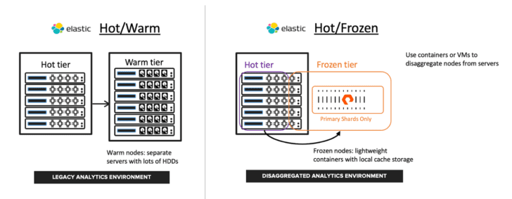
A hot/warm elasticsearch cluster traditionally uses performant flash storage for the hot tier with slower and cheaper spinning disks for the warm tier. The hot tier provides good ingest performance, which itself is an I/O intensive workload due to translog writes and periodic Lucene segment merges. The warm tier trades query performance for lower-cost data retention. Larger data sets require increasing node counts, adding more compute, memory, and storage. Higher node counts add to operational complexity due to more frequent rebalances and longer upgrade cycles. As an example of operational overhead, to increase retention requires not only adding more warm nodes but also rebalancing shards in order to take advantage of that new storage.
In contrast, the frozen tier disaggregates compute and storage for the non-hot data; the hot tier stays the same, but now historical data is moved to an object store such as FlashBlade. This application-aware disaggregation simplifies elasticsearch in the following ways:
- Replica shards are not needed on the frozen tier anymore because the object store is responsible for ensuring data durability and reliability. This at least halves the actual storage required.
- Fewer frozen nodes are needed because now node count sizing is done for query performance instead of fitting physical drives in servers to meet capacity requirements.
- Frozen nodes are lightweight, meaning that scaling operations and node failures are now effectively no-ops because frozen tier rebalancing simply updates pointers to the data on the object store.
An Elastic frozen tier significantly lowers costs at scale by reducing the number of data nodes needed and operational complexity by limiting the amount of data that needs to be rebalanced when scaling or handling node failures. Further, the hot and frozen nodes can coexist on the same physical servers, as shown in the diagram above, because frozen tier data reliability is handled by the object store and not the local server.
The pipeline architecture evaluated here builds on my previously presented disaggregated log analytics pipeline, which includes a very similar disaggregation of Confluent Kafka with Tiered Storage.
Configuring a Frozen Tier
There are two main steps to configure and use a frozen tier: First, create a snapshot repository backed by S3, and second, configure an index lifecycle policy with a frozen tier backed by that snapshot repository. The steps below configure everything using Kubernetes and Elastic Cloud for Kubernetes though they can be configured in any Elastic deployment model.
Configure Snapshot Repository
The first step is to configure a snapshot repository on S3 object storage, identical as if configuring a standard snapshot repository used for backup purposes.
The ‘repository-s3’ plugin needs to be installed to enable the snapshot repository code to speak to an S3 backend. In Kubernetes, this can be done either by building custom images or using an initContainer. The initContainer to install the plugin looks like this:
initContainers:
- name: install-plugins
command:
- sh
- -c
- bin/elasticsearch-plugin install --batch repository-s3
The alternate approach of building a custom container image with the plugin already installed also avoids the need to pull software from the internet on each pod’s startup. An example Dockerfile with the s3 plugin would be:
FROM docker.elastic.co/elasticsearch/elasticsearch:7.15.1
RUN bin/elasticsearch-plugin install --batch repository-s3
I also use an initContainer to populate the elasticsearch keystore with S3 credentials. The initContainer uses keys from environment variables and adds them to the keystore. As a result, the access keys are not visible as environment variables in the long-lived primary elasticsearch container.
initContainers:
- name: add-access-keys
env:
- name: AWS_ACCESS_KEY_ID
valueFrom:
secretKeyRef:
name: {{ .Release.Name }}-elastic-s3-keys
key: access-key
- name: AWS_SECRET_ACCESS_KEY
valueFrom:
secretKeyRef:
name: {{ .Release.Name }}-elastic-s3-keys
key: secret-key
command:
- sh
- -c
- |
env | grep AWS_ACCESS_KEY_ID | awk -F= '{print $2}' | bin/elasticsearch-keystore add --stdin --force s3.client.default.access_key
env | grep AWS_SECRET_ACCESS_KEY | awk -F= '{print $2}' | bin/elasticsearch-keystore add --stdin --force s3.client.default.secret_key
Now, elasticsearch should be able to connect to any S3-compatible backend to establish a repository. In non-Kubernetes environments, the “elasticsearch-plugin” and “elasticsearch-keystore” commands can be run directly on the elasticsearch hosts.
Next, the bucket for the snapshot repository needs to be created. This can be done either through the FlashBlade GUI/CLI or with other command-line tools like the aws-cli or s5cmd.
> s5cmd --endpoint-url https://10.1.1.1 mb s3://myfrozentier
Finally, configure the snapshot repository with a REST API call to elasticsearch. The example below creates a repository named “fb_s3_repository.” Replace the templated parameters of bucket name and S3 endpoint with values for your environment.
curl -sS -u elastic:$(ELASTICSEARCH_PASSWORD) -k -X PUT https://{{ .Release.Name }}-es-http:9200/_snapshot/fb_s3_repository?pretty -H 'Content-Type: application/json' -d
'{
"type": "s3",
"settings": {
"bucket": "{{ .Release.Name }}-myfrozentier",
"endpoint": "{{ .Values.flashblade.datavip }}",
"protocol": "http",
"path_style_access:" "true",
"max_restore_bytes_per_sec": "1gb",
"max_snapshot_bytes_per_sec": "200mb"
}
}'
The max_restore_bytes_per_sec needs to be faster than the default range of 40MB/s-250MB/s in order to allow searches to the frozen tier to utilize FlashBlade’s performance. I set the snapshot speed to a lower value than restore speed to avoid large drops in ingest performance during the snapshot operation.
Finally, my setup disables SSL by setting the protocol to “http” instead of “https” for simplicity; load a certificate into FlashBlade for full TLS support.
Verify Repository
Once configured, elasticsearch provides two APIs to validate snapshot repository connectivity and performance.
The snapshot verify command validates that all nodes can access the repository.
POST /_snapshot/fb_s3_searchable/_verify
An example response indicating success:
{
"nodes" : {
"A4d-DhvsSj6ASMCwugsTsQ" : {
"name" : "kites-es-all-nodes-pure-block-3"
},
"7mBxI_lET1GYexAm5lGFOQ" : {
"name" : "kites-es-all-nodes-pure-block-2"
},
"QnsxvpveQJy4nu6s3QPGZQ" : {
"name" : "kites-es-all-nodes-pure-block-0"
},
"bs2PO2tOQ6G62dT271RYLA" : {
"name" : "kites-es-all-nodes-pure-block-1"
},
"KkT8T4qPT2ue9JSc4MJkpA" : {
"name" : "kites-es-all-nodes-pure-block-4"
}
}
}
Elasticsearch also includes a repository analysis API to benchmark the snapshot repository backend and measure performance. Due to the longer running time (~6 minutes for me with the suggest parameters), I was not able to run this command through Kibana “Dev Tool,” so I instead used curl and jq directly:
curl -Ss -u "elastic:$PASSWORD" -X POST -k "https://kites-es-http:9200/_snapshot/fb_s3_searchable/_analyze?blob_count=2000&max_blob_size=2gb&max_total_data_size=1tb&concurrency=40&timeout=1200s" | jq .
Elasticsearch then runs a distributed benchmark to measure read, write, listing, and delete speeds. The screenshot below shows the load generated against FlashBlade S3 with a 5 node cluster:
This snapshot repository could now be used for a snapshot policy, and in the next section we configure a frozen tier backed by this repository.
Configure Frozen Tier
Elastic data tiers provide the flexibility to set policies and configurations to make performance/capacity trade-offs for large data sets. Nodes participate in tiers based on their configured “roles,” so to use the frozen tier we also need nodes with the “data_frozen” role.
Ensure you have designated some data nodes as being part of the “frozen” role with the following parameter:
node.roles: ["data_frozen"]
These nodes can also be part of other tiers, but dedicated nodes are encouraged to enable flexible allocation of resources and QoS across tiers.
The shared snapshot cache size represents the amount of local storage needed for the frozen nodes to use as a persistent cache, directly improving frozen tier query performance.
xpack.searchable.snapshot.shared_cache.size: "16gb"
Then create an Index Lifecycle Management (ILM) policy with a “frozen” phase. The example below creates a policy “filebeat” that rolls over indices from hot to frozen after the primary shards reach 50GB or 1 day.
curl -sS -u elastic:$(ELASTICSEARCH_PASSWORD) -k -X PUT https://{{ .Release.Name }}-es-http:9200/_ilm/policy/filebeat?pretty -H 'Content-Type: application/json' -d
'{
"policy": {
"phases" : {
"hot" : {
"actions" : {
"rollover" : {
"max_age" : "24h",
"max_primary_shard_size" : "50gb"
},
"forcemerge" : {
"max_num_segments" : 1
}
}
},
"frozen" : {
"min_age" : "1h",
"actions" : {
"searchable_snapshot": {
"snapshot_repository" : "fb_s3_searchable“
}
}
},
"delete" : {
"min_age" : "60d",
"actions" : {
"delete" : { }
}
}
}
}
}'
When dealing with a high-performance object store like FlashBlade, I also increase the thread pool sizes for snapshot and forcemerge operations:
thread_pool.snapshot.max: 8
thread_pool.force_merge.size: 8
Query Performance Test
Responsive queries are critical for historical data, often following the mantra “you don’t know what data you’ll need to retrieve, but you know it’ll be important when it’s time to search it.” In fact, if data is only being kept for long-term retention requirements without the need to access it, it should not be in Elasticsearch anymore at all!
This test setup was inspired by the performance results blogged about previously by Elastic.
Test data is synthetic weblog data from flog in JSON mode. To see an example of what this type of data looks like, the following command outputs one randomly generated line:
> docker run -it --rm mingrammer/flog -f json -n 1
{“host”:”242.91.105.103", “user-identifier”:”-”, “datetime”:”11/Sep/2021:11:00:39 +0000", “method”: “PATCH”, “request”: “/scalable/harness/plug-and-play/interfaces”, “protocol”:”HTTP/1.0", “status”:205, “bytes”:16760, “referer”: “https://www.centralout-of-the-box.info/incubate"}
Test Environment Details
Common application environment:
- Elasticsearch 7.12.1
- Two cluster sizes tested: 4 nodes and 8 nodes
- Nodes are both hot and frozen role, no concurrent ingest
- Rate limits set at 1GB/s per node
- Searchable snapshot cache at 1GB/node in order to focus on cache misses
- Simple match query across all indices
FlashBlade S3 Environment
- 8 nodes: 16 cores, 32GB, 7-year-old CPUs
- 12x 8TB blade system, Purity 3.2.0
- Kubernetes v19.0
- Total index data in frozen tier is 4.8TB
AWS S3 Environment
- 8 nodes m5.8xlarge
- EKS Kubernetes v19.6
- Total index data in frozen tier is 4.5TB
- Queries 2x slower if not tuning max_concurrent_shard_requests
Queries run in isolation, i.e., no concurrent ingest, across the entire data set and are designed to miss in cache in order to exercise the S3 snapshot repository.
The query used in testing was:
GET /_search?max_concurrent_shard_requests=50
{
"timeout": "120s",
"query": {
"match": {
"message": {
"query": "searching for $randomstring"
}
}
}
}
Results
Queries against the FlashBlade frozen tier were on average 3x faster than against AWS S3 in cache miss scenarios (and the same with cache hits). The performance gain grew larger for FlashBlade in the 8 node cluster.

The 8 node query briefly hits max expected FB throughput, meaning that increasing the number of blades will also improve query response time.
In neither case did performance increase linearly as cluster size grew from 4 nodes to 8 nodes, but it was much closer to linear on FlashBlade (83% faster) as opposed to AWS S3 (29% faster).
Parameters Tuned
The following parameters are relevant to the query performance results presented above.
xpack.searchable.snapshot.shared_cache.size=1GB: strong impact on query performance. With larger cache, the first query is slower, but then subsequent queries are faster. As this test focuses on cache misses in order to highlight the object store backend, this setting was set artificially low to 1GB.
max_concurrent_shard_requests=50. Setting to 50 from the default of 4 results in a 2x improvement on the AWS environment. On FlashBlade, this setting does impact the max read throughput observed on FlashBlade but does not improve the overall query response time.
indices.recovery.max_bytes_per_sec=1gb: a per-node setting that directly impacts how quickly data can be retrieved from the snapshot repository backend.
max_restore_bytes_per_sec=1gb: a snapshot repository setting with the default value of between 40MB/s and 250MB/s artificially slows down queries against fast object storage.
Deeper Dive into the Frozen Tier
Rollover
Data is written to the frozen tier when indices are “rolled over.” Under the hood, the rollover operation is equivalent to taking a snapshot of the completed index and then removing it from local storage. This has the great benefit of 1) not introducing any new code paths for the frozen tier write path, 2) allowing standard snapshot restore operations, as well as 3) mounting indices as a searchable snapshot from a different cluster.
The Kibana Stack Management UI makes it easy to navigate through the snapshots and restore to a new index.

The key here is that the data in the frozen tier can be used for dev/test scenarios by either cloning indices via restores into a new cluster or remotely searching indices via the snapshot mount command. A mounted snapshot allows searching from multiple clusters without making copies of the data set.
Restore and mount operations can happen in separate clusters configured with the same snapshot repository backend. The result would be a cloned cluster that could be used for dev/test purposes or a temporary search cluster for bursts of queries.
Query
Digging deeper into what happens during a query to the frozen tier, the elasticsearch API provides detailed statistics at the following endpoint:
GET /_searchable_snapshots/stats
Which breaks out statistics across individual types of files that make up the Lucene indices stored on S3 object storage. As an example, it shows total bytes read statistics as per this snippet of the JSON response:
"blob_store_bytes_requested" : {
"count" : 24,
"sum" : 201338880,
"min" : 1024,
"max" : 16777216
},
With these statistics, I can also tell that most of the data written to the local cache is from the term dictionary (“.tim” files) and term index (“.tip” files).
"cached_bytes_written" : {
"count" : 36,
"sum" : 402665472,
"min" : 1024,
"max" : 16777216,
"time_in_nanos" : 1943556975
},
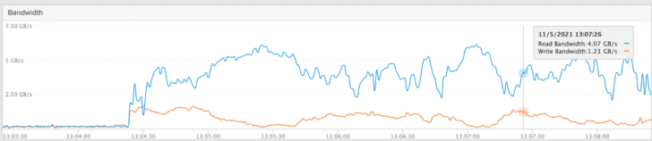
Another way to get insight into the I/O generated during a query that hits the frozen tier is to view the performance graphs from the storage perspective. The read burst of slightly under 6GB/s corresponds to the limit for this small FlashBlade. Increasing the size of the FlashBlade would offer linear scaling of this upper limit and improved query response times (assuming larger indices).
Reads from frozen tier S3 during query
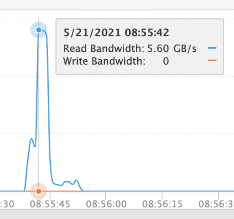
A second graph shows the corresponding writes to the local persistent caches aggregated across all nodes. Roughly 1/10 of data read is then written to the cache, i.e., only a subset of the index structures are written to the cache so that even small cache sizes are used effectively and not thrashed by large scans.

Writes to searchable snapshot shared cache during query
These graphs indicate that elasticsearch is able to query the S3 backend with high performance even with low numbers of data nodes, i.e., 6GB/s query with 8 nodes, as well as intelligently store subsets of the index structures on a local cache for higher performance on subsequent queries.
Summary
Elastic’s new frozen tier enables elasticsearch clusters to grow beyond 100TB scale and into PB scale by disaggregation of compute and storage. The frozen tier leverages an object store instead of node-local storage, enabling simpler scaling and failure handling and reducing capacity requirements. With FlashBlade S3 as the object backend, managing and scaling storage is install-and-forget simple, and queries against the frozen tier deliver the performance needed to leverage historical data when it’s inevitably needed.
![]()