
The Meta Workload Planner was publicly released as part of Pure1 on July 13, 2017. Get the latest on Pure1 Meta.
“Most of you don’t know me….let’s keep it that way”, was an opening remark that I delivered to a room full of Pure Sales Engineers. Back then I was in charge of handling SEV-1 cases with the Pure FlashArray. The talk was about the new Fingerprint Engine that we were building. It would enable predictive support and make my SEV-1 fighting role much less relevant. The time I spent handling SEV-1s deeply shaped me and the technology that I wanted to build. First and foremost on the priority list was eliminating any issues that were the fault of the FlashArray, that’s where the Fingerprint Engine comes in.
Next on that list, was helping customers get the most out of the array and get a better understanding of their workloads, that’s where the Pure1® Meta Workload Planner comes in.

Meta Workload Planner in Pure1
Imagine you are driving down a road and you know there is a cliff somewhere in front of you. Imagine further that the only way to tell if you reached the cliff is if you start falling. Accidents are bound to happen. In the early days of the FlashArray the only way to know if you were exceeding the “performance limit” of the array was if the IO latency began to spike. Accidents were bound to happen.
At first blush reporting the “performance limit” of the array seems easy and straightforward. Why not just report the CPU usage on the array? Well, unlike predicting capacity, there is no unique measure that can be used for performance sizing. For instance, with FlashArray the CPU usage is 100% all the time. The only difference between a heavily loaded array and one that is idle is which processes are causing the 100% CPU usage. In the heavily loaded case it’s the processes responsible for serving IO. In the idle case it’s processes that are optimizing the data already on the array to increase data reduction and optimize the metadata for ever-faster IO. In storage, predicting performance has always been a challenge because there could be hundreds of interacting variables and the math is very complex.
At Pure we believe in simplicity so we asked ourselves, can we condense these complex interactions that play into an array’s performance into the simplest form possible. One number, which we call the “load” of the array. The “load” would represent a distillation of busyness and utilization of all the subsystems that make up the array, and give the user actionable data.
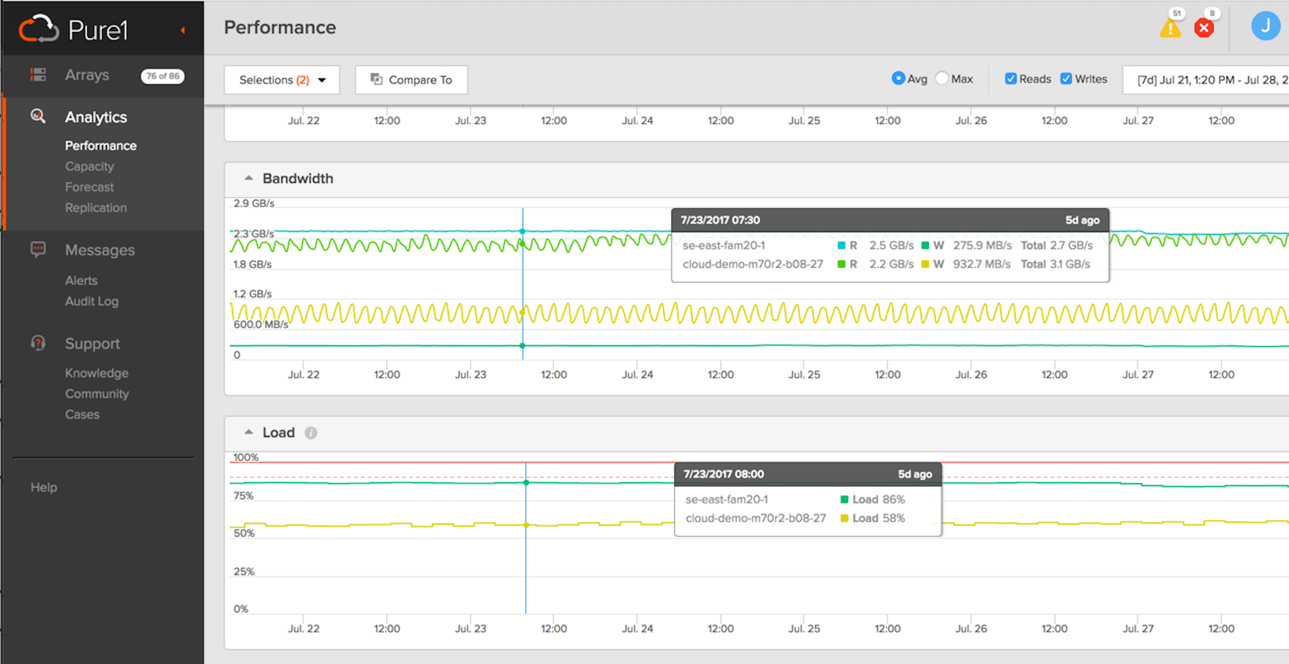
Array load is one of the performance metrics available in Pure1
This was a major step forward. Now customers knew how close they had driven to edge of the cliff in the past. There were, however, two major limitations with the first approach of computing load. First, it could not be projected into the future. Using the ratio of which processes were using the CPU to calculate load required data on per process CPU usage. The only way to get that data was to run the workload. There is no way to say, “what would happen if my workload grew 20%?” Since load is not linear, growing the workload by 20% will not necessarily increase the load by 20%. So the only way to know what would happen if you grew the workload by 20% is to try it. This lack of future prediction or “what-if” analysis is the first major limitation. The second limitation is that it is impossible to tell how the different workloads on the array contribute to the total load. Load is calculated as an array wide metric. Suppose the array is running a mix of VDI and SQL and suppose the load is 55. How much of that 55 is from the SQL? It is not possible to extract that information from the ratio of process run times.
Here we decided to look past the traditional modeling systems, and instead turn to our biggest asset, the data we have in Pure1. Our arrays constantly phone home telemetry data that captures thousands of sensor inputs about the array’s performance. Perhaps we could use this data to get a better insight into the performance of the array. Specifically, the question we sought to answer was how an array’s performance changes in response to the workload being run on it.
This led us to focus on phoned home metrics that are projectable and separable. An example of a metric that is both predictable and separable is “write IOPS”. If you know the write IOPS that were sent to this array over the last 6 months you can make a very good guess (projection) of the write IOPS for the next 6 months – that’s projectable. If you have 2 workloads on the array a VDI and SQL you can also easily separate the write IOPS that are coming from each of the workloads – that’s separable. Using only metrics that meet these criteria means that we will be able to project the load and separate the load for the different workloads thus overcoming the limitations of the previous method.
This now becomes a classic machine learning problem. We have a ton of data. Each data point consists of the input metrics like write IOPS which are called features in ML terminology. For each data point we also know the true load of the array at that time, the observation. We break the data points into two parts: a training set and a test set. We feed the training set into various machine learning algorithms that use this data to construct models. A model is a mathematical generalization of the data that takes features as input and predicts the load. We then test each of the different models on the training set (data that the model has not seen before) and compare the load predicted by the model with the true load that was observed. The model that gives the best results is selected. A similar process is used to fine tune and improve the accuracy of the champion model to make it even better.
The Meta Workload Planner was publicly released as part of Pure1 on July 13, 2017. It is the first tool utilizing the above mentioned models to predict load. When a user selects an array they will see its load over the last 1, 3, or 6 months (depending on window selection). This historic load was calculated by the original load calculation method. They will also see a projection of load into the future. This future load is calculated using the new machine learning models.
What is happening under the hood is that for the selected historical period we extract the past values of the input features. We project each of the features forward by first decomposing them into the daily and weekly seasonalities and extracting the underlying trend. We project the trends and return the seasonalities.
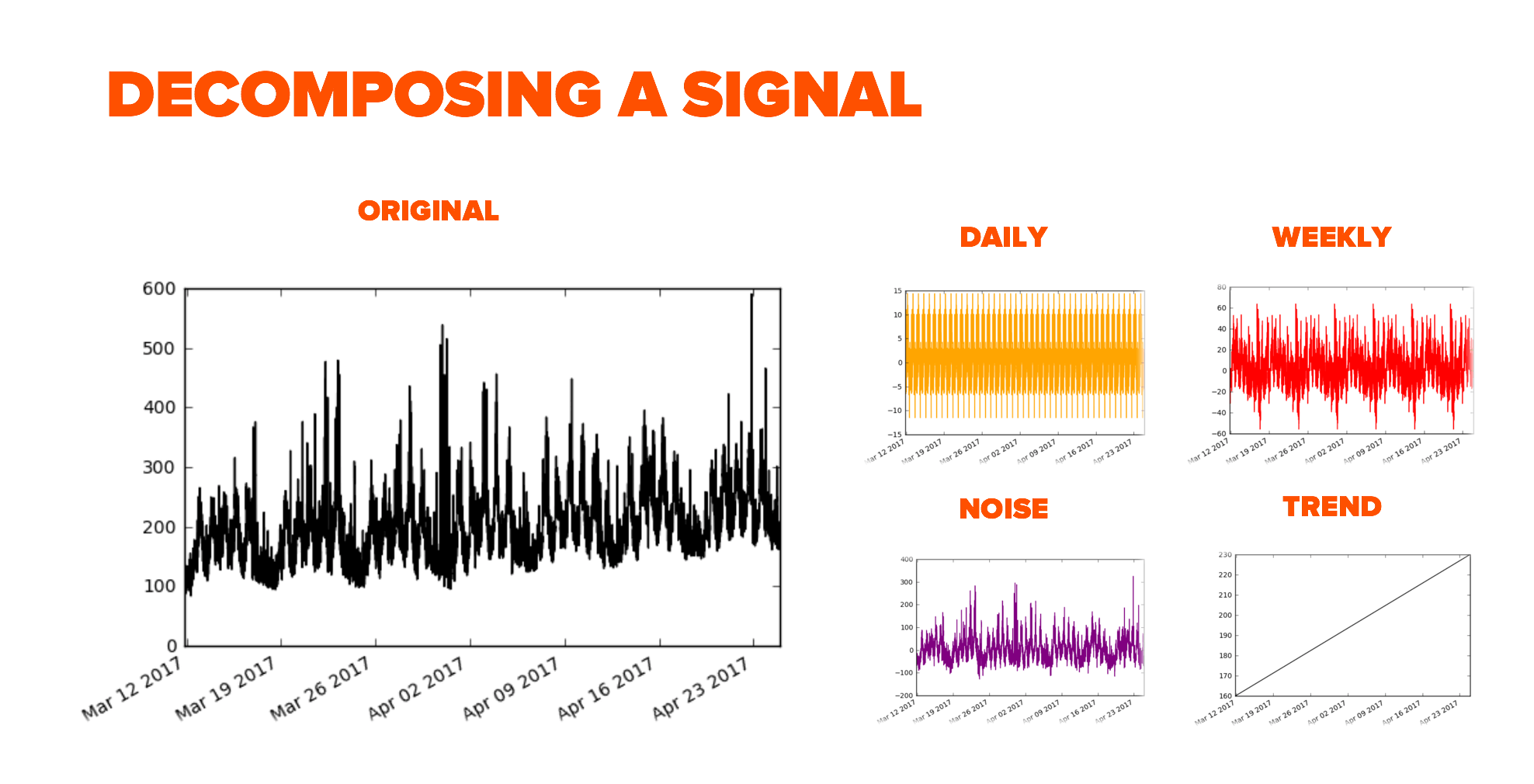
Once we have successfully projected all the input features into the future we feed these new data points into our model to calculate the future load which we display in real time in Pure1.
The real power of the above described methods are that the feature projections are specific to the array in question while the models gain tremendous accuracy by combining the knowledge and experience of every customer array in the field. We collect over a trillion data points per day from all our arrays and have seen probably every performance recording from any type of setup.
We continue to work on Meta and one of the possible next steps is view load per workload rather than array.

Our team of Pure1 engineers and data scientists
Stay tuned for more blogs on Pure1 Meta and how we are using machine learning to deliver on our vision of self-driving storage.